Special Courses
Applied Intertemporal Optimization
Lecturer: Prof. Dr. Klaus Wälde (Johannes Gutenberg-Universität Mainz)
Date: March 14, 2011 – March 17, 2011 (Universität Leipzig), daily at 9:30
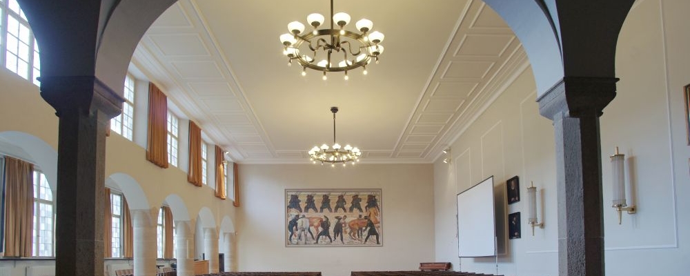
Venue: Universität Leipzig, Grimmaische Straße 12, Institutsgebäude, Room: SR 8 (I132)
Registration: sprenger@wifa.uni-leipzig.de
Course Description
The course will focus on making students familiar with one of the most widely used technique to solve maximization problems – which is dynamic programming. We will get to know dynamic programming methods and the corresponding Bellman equation first in the simplest possible setup, i.e. in discrete time and deterministic worlds. After some applications, we will move to dynamic programming in continuous time. Again, some applications will illustrate the pros (and the few cons) of this approach.
We will then proceed to get to know dynamic programming methods in setups where the method „feels at home“, where it can present all of its strenghts: in stochastic worlds. Starting again with discrete time and some applications, we will then focus on continuous time setups. Under continuous time and uncertainty, dynamic programming is basically the only simple-to-use method which allows to solve maximization problems. Continuous time uncertainty is widely used in macro, labour economics, resource economics, finance and, most interestingly for applications, for structural estimation.
In order to prepare the field for dynamic programming, we will go through two preliminary steps: We first learn what stochastic differential equations are and then talk about how to compute differentials in continuous time under uncertainty (i.e. we get to know Ito’s Lemma and its extensions for jump processes). After that, applications to economic maximization problems abound and there are no further limits to knowledge, wisdom and eternal happiness.
Time Schedule
Monday
09:30 – 11:00: Lecture 1
11:30 – 13:00: Lecture 2
16:00 – 17:30: Lecture 3
Tuesday
09:30 – 11:00: Problem Sets
11:30 – 13:00: Lecture 4
16:00 – 17:30: Problem Sets
Wednesday
09:30 – 11:00: Lecture 5
11:30 – 13:00: Lecture 6
16:00 – 17:30: Problem Sets
Thursday
09:30 – 11:00: Lecture 7
11:30 – 13:00: Lecture 8
16:00 – 17:30: Problem Sets
Further Information
The lectures will present selected material from the textbook Applied Intertemporal Optimization freely available for download at www.waelde.com/aio.
Part I and IIWe will start with ch. 3 (up to p. 56) where we use dynamic programming for solving a discrete time deterministic model. We then make rapid progress by ignoring ch. 4 (assuming that there is a certain familiarity with ordinary differential equations) and, with the exception of ch. 5.1, all the rest of ch. 5 (which is on optimal control theory/ Hamiltonians). We do treat ch. 5.1 as it is useful for later comparison purposes. We continue more slowely with ch. 6 (up to p. 145) where we employ dynamic programming again to solve a deterministic continuous time problem.
Part III and IV
The next chapter will be ch. 7.4.1 which illustrates the basic difference between deterministic and stochastic models. Models no longer predict the evolution of one or several variables but of one or several distributions of variables. Dynamic programming will then be used again in ch. 9.1 and 9.2. Ch. 9.5.1 then shows how you can live very well without dynamic programming.
If time permits, we will then get to know the most fascinating field of stochastic worlds: Continuous time stochastics. This will start in ch. 10 and will continue with optimization problems in ch. 11. We will see during the week how to structure these two chapters.
Sessions entitled „Problem Sets“ will go through following problem sets:
Part I and II
Ch.3 ex. 2, 5, 7(a,b,c)
Ch.5 ex. 1, 4, 5
Ch.6 ex. 1
Part III and IV
Ch.7 ex. 4, 5
Ch.9 ex. 5, 8
Ch. 10 ex. 2, 3a, 4, 7a, 10a
Ch.11 ex. 1, 3(a,d), 4,
which will be solved in class.
Further information on the Short Course you can find here.
